Table of Contents
Scientific background of the Modular Megafauna Model.
Introduction
This document explains the design choices for the modules and concepts in the megafauna model from a scientific rather than a programmatical angle. It discusses the different submodels in the framework: what their assumptions are, how to use them, and how to combine them.
Because of the modular nature of the software, you can “generate” a range of models with different combinations and configurations of submodels. Therefore this documentation page must not be seen as a “model description”, but rather as a loose discussion of available model components. It is a living document that ought to be expanded when new features are introduced to the library.
The first section, Model Goals, shall help you clarify the direction of your modeling project. The section Basic Model Concepts introduces the simulation framework of the Modular Megafauna Model: where it is flexible and where it is constrained. The following sections describe conceptual elements of the Dynamic Populations, which are currently represented by the herbivore type “cohort,” and conclude with some lessons learned from emerging model behavior. At the end of this document, you will find a list of Symbols and Abbreviations and a remark on the choice of Units of Measurement in the model.
Some aspects of the model can only be evaluated in the context of the connected vegetation model. For LPJ-GUESS you will find those aspects in the megafauna doxygen page of the LPJ-GUESS repository.
Model Goals
Before you start your modeling project, you should have your model goal defined. The formulation of the model goal paints in broad strokes a picture of the direction you want to take. In the next step, the definition of a model purpose will help you convert the goal statement into an objective statement. The objective is more concrete than the goal and can be further refined into model specifications, which serve as reference points for evaluating the output of your model candidates and whether you have reached your goal. For a more more detailed discussion of these terms see Overton (1990)[46].
The Modular Megafauna Model, by its flexible nature, shall serve as broad of a range of model goals as possible. Its modularity is supposed to help in the iterative modeling process. You can combine different submodels to create a number of different intermediate developmental models. They can then be evaluated against your model specifications. When composing your model, be wary of the “complexity paradox”: The more complex (i.e. “realistic”) your model is, the more uncertain it is and the more difficult it is to know if your tests of the model are meaningful (Oreskes 2003[45]).
The only goal given by the software architecture of the Modular Megafauna Model can be stated thus: to simulate herbivore–vegetation dynamics over time. By selecting model components, the goal becomes more specific, and so the herbivore type “cohort” (see Section Herbivore Cohorts) has the goal to dynamically simulate herbivore population densities as they emerge from basic mechanistic processes. Herbivore densities are not prescribed, but emerge bottom-up. Based on that, project-specific model objective statements can be formulated, for instance, “to simulate bison populations in the North American prairie for the purpose of estimating potential pre-European carrying capacity.” The model components must then be selected or newly implemented to meet that objective. In North America, for example snow cover may play a role and should be included in the model. If the objective were to simulate wildebeest in the Serengeti, snow wouldn’t play a role and should be excluded from the model.
Therefore, before you start working with the Modular Megafauna Model, gain as much clarity as possible about your model goals, purposes, objectives, and specifications. You might even want to consider a preregistration, see for example Nosek et al. (2018)[44], Lee et al. (2019)[39], and Dirnagl (2020)[13].
Basic Model Concepts
The world of the megafauna model is comprised of simulation units. Each such unit consists of a habitat and the herbivore populations inhabiting it. The habitat must be implemented by the outside vegetation model. Output can be spatially aggregated over several habitats by assigning multiple habitats to the same aggregation unit. Again, this is done by the habitat implementation of the vegetation model. What kind of herbivores populate the world can be defined by the user. Cohorts are the first herbivore type implemented.
For the megafauna model, all habitats are of equal size and spatially inexplicit. Spatial meaning must be given by the outside vegetation model; for example LPJ-GUESS maps each grid cell in the longitude/latitude raster to one aggregation unit. Currently, there is no interaction between habitats, that is herbivores cannot move from one to the other. Each habitat can be thought of as a little homogeneous capsulated world of forage and herbivores.
The simulations run with daily time steps. The predecessor model by Adrian Pachzelt [49] operated on a monthly schedule and was thus much faster. However, the Modular Megafauna Model should be applicable on different spatial and temporal scales. LPJ-GUESS simulates vegetation in a daily schedule, and so naturally the attached herbivores should be treated the same. Moreover, there has been no formal analysis how much a coarser temporal resolution affects the model outcome. So it seemed better to air on the side of a finer resolution.
The vegetation model makes plant biomass available to herbivores as dry matter forage mass per area. The megafauna model works with a hard-coded set of forage types, for example “grass.” It is up to the vegetation model to map its own representation of edible biomass to forage types, for instance by aggregating all graminoids, herbs, and forbs to one “grass” forage mass. The advantage of this approach is that the herbivore model is highly decoupled from the vegetation model. Placing forage types as hard-coded entities at the core of the herbivore model makes it easy to design herbivore diet preferences, foraging, and digestion around them. New forage types can be implemented as necessary.
Dynamic Populations
Herbivore Cohorts
A cohort represents all herbivores born in one year. The state variables of a cohort represent an average over all individual animals within the cohort. The main reason to not simulate individuals is to save computational resources.
These are the state variables for each herbivore object:
- Age
- Sex
- Current energy need
- Fat mass
Each herbivore cohort is assigned a herbivore functional type (HFT). The HFT can be interpreted as representing a species, a guild, or a trophic level. An HFT is simply a user-defined, constant set of parameters defining physiology, life history, and everything else. Each cohort population contains all cohorts of one HFT in a particular habitat. Therefore, the maximum number of cohorts within one population is given by the HFT life span in years times two, for the two sexes.
Offspring of large herbivores usually shows an even sex ratio. Most model processes don’t differentiate between males and females, only body size and age of maturity have sex-specific parameters. During the model design, it seemed advisable to at least set the basis for gender differentiation because some large herbivores do show pronounced sexual dimorphism not only in size (e.g. bison or proboscideans) but also in diet and behavior (e.g. elephants, Shannon et al. (2013)[60], and steppe bison, Guthrie (1990)[22]).
Each year, the newborn animals of all reproductive cohorts of one HFT in one habitat are combined into one new cohort. This effectively eliminates the connection between parents and offspring. Therefore it is not possible to implement an exchange of energy through lactation between parents and young directly.
Body Mass and Composition
The user-defined live body mass of simulated herbivores is the sum of blood, gut contents (ingesta), structural (fat-free) mass and deposited body fat. It is very important to realize that the body fat that the model works with is the fraction of fat in the empty body. The empty body mass is the live body mass minus blood, ingesta, hair, and antlers/horns. The body fat is total lipid content, which is also known as ether extract, free lipid content, or crude fat (Hyvönen, 1996 [30]). This is different from the mass of suet and organ fat because the fat tissue also contains water. The term lean body mass is live body mass minus all fat mass (compare quote from Blaxter, 1989 [4] in Section Fat as Energy Storage). Note that lean body mass includes digesta, hair, antlers, and blood.
Calder (1996, p. 14) [7] discusses the question of variable ingesta load:
Should the total body mass used in allometry include gut contents, a major source of variability (but representing mass that the animal must be designed to support and carry), or should gut contents be subtracted from live mass? Disallowing gut contents is not practical in studies wherein the animals are not, or should not be sacrificed.
In this line of argument, the gut contents are always included the body mass values given in the megafauna model. It is designed for large herbivores, in particular extinct ones, and their body mass is most commonly given as a total live weight. Live body mass is easy to measure. Most allometric regressions are based on it.
Technically, the empty body mass is different from the “ingesta-free mass” in the literature because ingesta-free mass usually includes hair. For less furry animals the two can be considered approximately equal, though.
Fat as Energy Storage
The variable amount of body fat, which serves as energy reserves, is a critical component of the herbivore simulations. As Blaxter (1989, p. 51) [4] explains, the ingesta-free animal body can be viewed as composed of fat and fat-free mass:
Schematically the body can be regarded as consisting of two components – fat and non-fat. […] The non-fat material consists of water, the minerals of bone and soft tissue, carbohydrate, nitrogen-containing compounds, and, in the living animal, the contents of the digestive tract. The non-fat component of the body is usually referred to as the lean body mass or fat-free mass. Many studies, commencing with those of Murray (1922) and embracing a wide range of adult species, have shown that the chemical composition of the fat-free body is approximately constant. The wide range of composition of animals is largely, but not entirely, due to variation in the proportion of fat.
When defining the fractional body fat parameter for an herbivore, you should not rely on measurements of weight loss of starving or fattening animals. In such data it is difficult to disentangle the contributions of changing fat mass, gut contents, water content, and fat-free mass (e.g. Reimers et al., 1982 [55]).
The model ignores the contribution of catabolizing protein altogether. This is a simplification as several studies have shown that the contribution of mobilized protein can play a considerable role in meeting energy requirements. Reimers et al. (1982, pp. 1813, 1819) [55] observe that reindeer lost about 31% of their body protein during winter. Torbit et al. (1988) [67] calculate and discuss the energetic value of catabolizing protein. Parker et al. (1993) [51] note that Sitka black-tailed deer lost 10–15% of their protein reserves during winter. Nontheless fat is unquestionably by far the most important energy reserve. Fluctuating body fat is convenient to model as an energy pool that can be filled to a maximum and emptied to zero. The interactions for protein synthesis and depletion are far more complex and less studied.
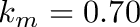
Any forage energy that is ingested beyond maintenance needs is converted to body fat. Section Energy Content of Forage details the efficiency of fat anabolism. When forage intake is not enough to meet energy needs, fat reserves are catabolized, and the energy is directly available as net energy to balance any energy “debts” on a daily basis. Illius & O’Connor (2000) [35] assumed an efficiency of 100% to mobilize fat reserves in cattle when they directly converted the combustion (gross) energy of fat tissue to net energy. Armstrong & Robertson (2000) [2] use a factor of 80% in their sheep model, citing a 1990 publication by the Australian Standing Committee on Agriculture (SCA) [10]. The megafauna model allows the catabolism efficiency to be specified by the user. This efficiency factor is multiplied with the fat gross energy to derive the net energy gain (MJ) from burning one kg of body fat.
Ontogenetic Growth
The growth curve is currently linear. The body mass of a cohort that hasn’t reached physical maturity yet is calculated as a linear interpolation between the user-defined neonate body mass and adult body mass. However, the growth curve should be sigmoid, compare Price (1985, pp. 187–190)[54] and this quote by Blaxter (1989)[4], p. 242f:
Growth in weight is characteristically sigmoid; it accelerates during a short initial period and then declines until, as maturity approaches, it approaches zero. A large number of different functions have been used to describe this relationship between weight and time. Virtually all of them state that dW/dt, the rate of change in weight with time (or rate of growth) is a function of weight at the time that dW/dt is measured. Such functions include the logistic equation, the Gompertz function and the Bertalanffy function. These are derived algebraically in most textbooks of biomathematics (see Causto 1977). They were generalised by F.J. Richards (1959) and have been reviewed and critically analysed by Parts (1982).
Energy Budget
Energy Expenditure
The allometric scaling of metabolic rate in the megafauna model does not differentiate between inter- and intraspecific scaling. This model assumption might need to be re-evaluated in the future. As Makarieva et al. [41] point out:
However, it has repeatedly been observed that young animals have elevated metabolic rates compared with what is predicted for their body mass from interspecific scaling (5–8).
Compare also Glazier (2005) [20] for a discussion on intraspecific metabolic scaling.
Energy Content of Forage
The model for energy content in herbivore forage presented here is based on the partitioning of metabolizable energy. A historical overview of the model framework is given by Ferrell & Oltjen (2008) [14]. Its conceptual shortcomings and difficulties in practical methodology are summarized by Birkett & de Lange (2001) [3].
The diagram on the energy budget shows how energy from the forage is used by an herbivore: Gross energy ( 


Gross energy depends only on the physical properties of the forage and measured in a combustion chamber. It is therefore independent of the animal. McDonald et al. (2010, p. 259)[42] provide an overview of gross energy in different feedstuffs for livestock: It typically ranges between 18 to 20 MJ/kgDM. The measurements by Golley (1961) [21] suggest that there is some seasonal variation in gross energy of leaves. However, the model assumes a constant value.
The proportional dry-matter digestibility ( 
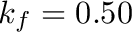
Research has focused mainly on the digestion of ruminant livestock, and so the megafauna model works primarily with the well-established formulas for ruminants. Digestibility is also defined for ruminants. To account for the less efficient digestion of hindgut fermenters, the user can define a digestibility multiplier to convert ruminant digestibility to hindgut digestibility. This approach is taken from by and Pachzelt et al. (2015) [50], who cite Illius & Gordon (1992) [33]
Ruminants typically lose a relatively constant fraction of about 19% of digestible energy in urine and methane (López et al. 2000 [40], McDonald et al. 2010 [42], p. 258). The difference between cattle and sheep is very small here (McDonald et al. 2010, p. 260). McDonald et al. (2010, p. 258) specify that 11–13 percent of digestible energy is lost as methane. The 19% loss to urine and gases is often expressed as the ratio of metabolizable energy to digestible energy, 
- Warning
- Some publication, like Minson (1990)[43], use the term “metabolizability of energy” or “metabolizable energy coefficient” to refer to the

A unitless net energy coefficient ( 


In the Modular Megafauna Model, the energy budget calculates with the “currency” net energy, which broadly represents the available oxidizable metabolic fuels—glucose and fatty acid. Basal and field metabolic rate and other energy expenditures are directly “paid” with net energy. Therefore the efficiency factor
Feeding trials have shown that the net energy coefficient can linearly depend on the metabolizable energy content of the forage (Robbins, 1983, p. 296f; Minson, 1990, p. 93, 155). However, this effect seems to be mostly related to very high levels of feeding and by pelleting the feed. In this model, the energy coefficients
- Remarks
- Internally the model converts first from metabolizable energy to net energy to pay energy expenditures. If there is excess net energy, this gets converted afterwards to body fat. The amount of net energy required to build up one kilogram of body fat is given by the product of fat gross energy content,


In summary: Net energy content, 
![\[
NE = ME * k_m = DE * \frac{ME}{DE} * k_m = GE * DMD * \frac{ME}{DE} * k_m
\]](form_96_dark.png)
Thermoregulation by Conductance
This model of thermoregulation is often called the Scholander-Irving model and was published in two seminal papers in 1950: Scholander et al. (1950a) [58] and Scholander et al. (1950b) [59]. The more detailed implementation is taken from Peters (1983) [53].
Homeothermic animals have extra energy costs to maintain their body core temperature. Through basal metabolism and other ways of energy burning, heat is already passively created. Thermoregulatory costs arise when the ambient temperature drops below the lower critical temperature: the passive heat from thermoneutral metabolism is not counterbalance heat loss to the environment. The rate of heat loss depends on the thermal conductance of the whole animal (energy flow per temperature difference), which in turn depends on the thermal conductivity (energy flow per temperature difference and per thickness) of fur and skin and the body surface. Conductance is the inverse of resistance or insulation, and conductivity is the inverse of resistivity.


![\[
T_{crit} = T_{core} - \frac{E_{neu}}{C}
\]](form_103_dark.png)
![\[
\Phi = C * max(T_{crit} - T_{air}, 0)
\]](form_104_dark.png)
- Note
- In its current form, the model only considers costs when temperatures are too low. Overheating effects are not implemented since the model was developed with the focus on Arctic megafauna.
The critical parameter for thermoregulatory expenditure is the whole-body conductance: the rate of heat flow per difference between core and air temperature (W/°C). The conductance can be approximated from the average conductivity and the body surface. Conductivity is the inverse of insulation: it is the heat flow per temperature difference per area.
Body surface in m² scales roughly as 
Foraging
An herbivore’s daily dry matter intake can be limited by any of a number of factors, as illustrated by the following figure:
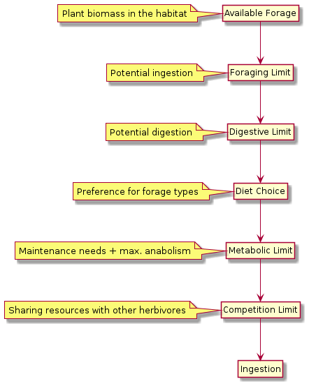
The functional response is the intake rate as a function of available forage (Holling 1959a[27]) and corresponds to the “foraging limit” in the megafauna model. Grazers are generally thought to have a Type II functional response (Owen-Smith 2002[47]): their intake rate quickly increases with increasing food abundance towards an asymptotic maximum. This maximum is the rate at which an herbivore could theoretically ingest forage if there were no constraints of forage abundance, digestive capacity, or metabolic requirements.
The Type II functional response is commonly expressed as a hyperbolically saturating function (Holling 1959b[28]), which is also known as “Michaelis–Menten” function in other contexts. The critical parameter of this function is the forage density at which the intake rate reaches half of its maximum. Owen-Smith (2002)[47] calls it 

- Note
- Illius and O’Connor (2000)[35] and subsequent similar models (e.g. Pachzelt et al. 2013[49]) use an empirically derived half-maximum intake density,

Following a seminal publication by Spalinger and Hobbs (1992)[64], a lot of work has been done to model the functional response of grazers mechanistically (e.g. Illius and Fitzgibbon 1994[31]; Bradbury et al. 1996[5]; Fortin et al. 2002[15]; Hobbs et al. 2003[26]; Fortin et al. 2004[16]; Robinson and Merrill 2012[57]). In the short term, grazers may be limited by encounter rate (moving between forage patches) or handling rate (cropping and chewing), which means they might not be able to ingest the amount of forage they desire even though there is enough forage available. However, in the long term (i.e. over days and months), the intake of grazers is most likely to be digestion-limited. That is because they can compensate encounter and handling limitation by increasing their daily foraging time. In other words, the functional response curve increases so sharply with even low forage density that it does not play a major role in the long term.
Mortality
Cohorts are deleted when they have reached their life span. The population numbers are gradually decreased with a user-specified annual background mortality and by starvation.
Death of Starvation
In the process of starvation, different fat depots are mobilized in a typical sequence: rump fat, subcutaneous fat, visceral fat, and, finally, marrow fat (Hanks, 2004/1981 [24]). When the energy reserves of an animal are exhausted, it will die of starvation. Body fat, i.e. lipid in the ingesta-free body, is then zero. Different studies have found that the carcasses of large herbivores that have starved to death contain virtually no body fat anymore (Reimers et al., 1982 [55]; Depperschmidt et al., 1987 [12]), but chemical analysis of fat content in carcass samples can be imprecise (Depperschmidt et al., 1987).
Population Dynamics
Population Stability
Several qualities of the model result in a propensity towards extreme instability of the simulated herbivore populations, with exponential irruptions followed by sudden crashes (sometimes to extinction). Here are some of the reasons for these “boom–bust cycles”:
- If there is no regular seasonal die-off, there is effectively no early density dependence effect. Herbivores just reproduce exponentially until the population crashes completely. In winter or the dry season, the fat storage should drop so far that a fraction of the population dies because then density dependence effects occur at those times when there is not enough forage in the vegetation period to completely fill all animals’ fat storage. Another controlling factor can be variable climate: long or harsh winters/dry seasons can also regulate the population and prevent uninterrupted exponential growth. See for example Stewart et al. (2005)[65] for a discussion of the roles of summer versus winter in regulating populations of large mammals.
- There is no resource heterogeneity, only grass. If there was more heterogeneity with low-quality and high-quality forage, populations might be more stable (Owen-Smith 2004[48]).
- There is no movement between habitats. That is, a crashing population has no way to escape extinction by moving somewhere else. The situation in each habitat is comparable to an island population (e.g. Klein 1968[37]).
- Annual grass allocation in the case of MMM being coupled with LPJ-GUESS: Since LPJ-GUESS allocates one year’s NPP at the end of the year (Dec. 31st), herbivores will have to starve until the end of the year when all forage is eaten.
For further discussion and brainstorming see also these excerpts from Wolfgang Traylor’s lab notebook on Open Science Framework:
- 2017-09 Why do Populations Crash?
- 2017-10 Christmas Present
- 2017-12 Coexistence and Stability
- 2018-02 Closeup on a Crash
- 2018-06 Fat, Stability, and Movement
Minimum Density Threshold
The parameter Fauna::Hft::mortality_minimum_density_threshold defines at which point a dwindling population (sum of all cohorts) may be considered dead. It is an arbitrary and artificial, but critical “tuning parameter” for realistic model performance. Possible re-establishment only happens if all cohorts are dead within one habitat.
It is important to keep this parameter low enough for slowly breeding and long-lived animals because otherwise they may die out after establishment: After establishment, the background mortality continually diminishes the adult cohorts, and after some years the total population (all cohorts together) my drop below the minimum_density_threshold before reproduction could compensate.
On the other hand, the minimum_density_threshold should not be set too low as this would result in extremely thin “ghost” populations that are effectively preventing re-establishment.
Species Coexistence
The classical competitive exclusion principle predicts that no two species can coexist in the long term if they each solely depend on one shared resource (Hardin 1960[25]). One species will inevitably outcompete the other one. Though there are indeed ecological mechanisms that can facilitate coexistence with a shared resource (Chesson 2000[9]), the parameter space for this to happen in a model is usually very narrow (e.g. van Langevelde et al. 2008[68]).
In order to simply avoid competition among different HFTs, the option Fauna::Parameters::one_hft_per_habitat can be enabled: Each HFT exists on its own, without any interaction with other species. With that option enabled, all HFTs should each be assigned to the same number of habitats. It is the responsibility of the host application (the vegetation model) to ensure that the number of habitats is an integer multiple of the HFT count.
Symbols and Abbreviations


- Subscript

- Subscript

- Subscript

- Subscript


- General subscripts:


Note that “mass” and “weight” are used interchangeably.
Units of Measurement
- All forage values (e.g. available grass biomass, consumed forage) are dry matter mass in kilograms (
DMkg). - Any forage per area (e.g. forage in a habitat) is
kgDM/km². - Herbivore-related mass values (e.g. body mass, fat mass) are also
kg, but live mass (see Body Mass and Composition). - Population densities of herbivores are either in
kg/km²orind/km²(“ind” = “individuals”). - Digestibility values are interpreted as in-vitro digestibility (see Energy Content of Forage).
- Remarks
- The units of measurement were primarily chosen in a way to yield numbers broadly around zero for calculation. Floating point operations are most precise then, and the values can be printed in a text output table. When post-processing the output, you can convert to your units of choice, e.g.
ind/hainstead ofind/km².
- Copyright
 This software documentation is licensed under a Creative Commons Attribution 4.0 International License.
- Date
- 2019